Gent
ConstitutiveModels.Gent — Type
struct Gent <: ConstitutiveModels.AbstractHyperelasticityConstitutiveModels.helmholtz_free_energy — Method
$\psi = \frac{1}{2}\left[\frac{1}{2}\left(J^2 - 1\right) - \ln J\right] - \frac{1}{2}\mu J_m\ln\left(1 - \frac{\bar{I}_1 - 3}{Jm}\right)$
helmholtz_free_energy(_::Gent, props, ∇u, θ) -> Any
ConstitutiveModels.initialize_props — Method
initialize_props(_::Gent, inputs::Dict{String}) -> Any
Simple Shear
Analytic Solution
$\mathbf{\sigma}_{11} = \frac{2}{3}\frac{J_m\mu\gamma^2}{J_m - \gamma^2}$
$\mathbf{\sigma}_{22} = -\frac{1}{3}\frac{J_m\mu\gamma^2}{J_m - \gamma^2}$
$\mathbf{\sigma}_{33} = \mathbf{\sigma_{22}}$
$\mathbf{\sigma}_{12} = \frac{J_m\mu\gamma}{J_m - \gamma^2}$
All other components are zero
Verification
Here is a comparison of an analytic solution to the uniaxial stress boundary value problem in displacement control.
using ConstitutiveModels
using Plots

function gent_simple_shear()
    inputs = Dict(
        "density"         => 1.0,
        "Young's modulus" => 1.0,#u"MPa",
        "Poisson's ratio" => 0.3,
        "Jm"              => 13.125
    )

    model = Hyperelastic(Gent())
    motion = SimpleShear(t -> t)
    out = simulate_material_point(cauchy_stress, model, inputs, motion, 1.0)

    props = initialize_props(model, inputs)
    ∇us = map(x -> x.kinematics, out)
    γs = map(x -> x[1, 2], ∇us)
    σs = map(x -> x.material_output, out)
    Zs = map(x -> x.state, out)

    μ, Jm = props[3], props[4]
    σ_11s_an = (2. / 3.) * Jm * μ * γs.^2 ./ (Jm .- γs.^2)
    σ_22s_an = -(1. / 3.) * Jm * μ * γs.^2 ./ (Jm .- γs.^2)
    σ_12s_an = Jm * μ * γs ./ (Jm .- γs.^2)

    plot(motion, ∇us, σs, Zs, σ_11s_an, σ_22s_an, σ_12s_an)
end
gent_simple_shear()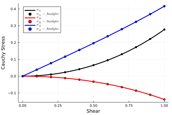
Uniaxial Strain
Analytic solution
$\mathbf{\sigma}_{11} = \frac{1}{2}\kappa\left(\lambda - \frac{1}{\lambda}\right) + \frac{2}{3}\mu\left(\lambda^2 - 1\right)\lambda^{-5/3}$
$\mathbf{\sigma}_{22} = \frac{1}{2}\kappa\left(\lambda - \frac{1}{\lambda}\right) - \frac{1}{3}\mu\left(\lambda^2 - 1\right)\lambda^{-5/3}$
$\mathbf{\sigma}_{33} = \mathbf{\sigma_{22}}$
All other components are zero.
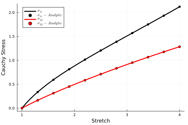
Verification
Here is a comparison of an analytic solution to the uniaxial stress boundary value problem in displacement control.
using ConstitutiveModels
using Plots

function gent_uniaxial_strain()
    inputs = Dict(
        "density"         => 1.0,
        "Young's modulus" => 1.0,#u"MPa",
        "Poisson's ratio" => 0.3,
        "Jm"              => 13.125
    )

    model = Hyperelastic(Gent())
    motion = UniaxialStrain(t -> 1 + 3t)
    out = simulate_material_point(cauchy_stress, model, inputs, motion, 1.0)
    props = initialize_props(model, inputs)
    ∇us = map(x -> x.kinematics, out)
    λs = map(x -> x[1, 1] + 1, ∇us)
    σs = map(x -> x.material_output, out)
    Zs = map(x -> x.state, out)

    κ, μ, Jm = props[2], props[3], props[4]

    σ_11s_an = 0.5 * κ .* (λs .- 1. ./ λs) -
               (2. / 3.) * Jm * μ .* (λs.^2 .- 1.) ./
               (λs.^3 - (Jm + 3) * λs.^(5. / 3.) + 2. * λs)
    σ_22s_an = 0.5 * κ .* (λs .- 1. ./ λs) +
               (1. / 3.) * Jm * μ .* (λs.^2 .- 1.) ./
               (λs.^3 - (Jm + 3) * λs.^(5. / 3.) + 2. * λs)

    plot(motion, ∇us, σs, Zs, σ_11s_an, σ_22s_an)
end
gent_uniaxial_strain()